How to Overcome Data Uncertainty in Water Quality Monitoring

Overcoming Water Quality Monitoring Data Uncertainty

Editor’s Note: The following transcript has been edited for readability.

Video Transcription

Transcript by Speechpad.

Nate: Hello, everyone, and thank you for joining us for our webinar about How to Overcome Data Uncertainty in Water Quality Monitoring.

In this webinar, our applications experts will share their guidance on how to overcome data uncertainty. They'll share insights into sensing technology commonly used in catchment monitoring, as well as sharing data from the field to show how best practices can help ensure data integrity over long-term deployments.

Let's go ahead and meet those experts. Darren Hanson is the Sales Director for Xylem UK. He has over 30 years of experience with senior scientists and water quality experts around the world. Up next is James Chapman, the Business Development Manager for Xylem UK. While he's new to us here at Xylem, he has over 13 years of experience in the industrial, municipal, wastewater, and environmental monitoring industries. We also have Catie Marchand on the webinar with us to help with the Question and Answer section. She's the Applications Engineer for some of our leading water quality instruments and has years of technical expertise in the field. And lastly, I'm Nate Christopher, Marketing Communications Manager, and I'll be your host for the webinar today.

This presentation will take approximately 45 minutes, and will cover major topics including an overview of the Environment Act 2021, as well as three case studies focused on water quality parameters and lab traceability, the impact of fouling on field instrumentation, and a closer look at complementary and derived parameters.

For now, I'll hand things over to James to get us started with an overview of the Environment Act 2021 and its impact.

Overview of Environment Act 2021

James: Thanks, Nate, for the introductions. Now, I'm sure we've all heard of the Environment Act by now, especially the water and environmental professionals within the UK. This is a world-leading Environment Act. It became law in November 2021. The legislation sets out to improve air and water quality, tackle waste, increase recycling, halt the decline of species, and improve our natural environment. For this webinar, we'll focus on water quality and the act's ambitious targets for the protection of our rivers and estuaries.

 

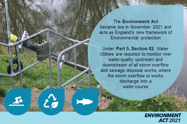
As you can see in the extract Part 5 Section 82 of the Act, it states, "All English water companies are required to continuously monitor water quality upstream and downstream of all sewage storm overflows and sewage treatment works discharging into a watercourse." On this slide, we see another extract from the Act, which states, "The water quality parameters required to be monitored are dissolved oxygen, temperature, pH, turbidity, ammonia, and anything else specified in the regulations made by the Secretary of State." The aim of this Act is to reduce the number of sewage-related spills in our rivers, lakes, and coastal areas, and improve overall water quality in our river catchments.

Current targets of the Act include the requirement to monitor at least 40% of all assets, i.e. sewage works and overflow discharge locations, which are not exempt by the end of AMP8, i.e. 2030. This includes all assets defined as high-priority sites, which include sites of special scientific interest (SSSIs), special areas of conservation (SAC), urban wastewater treatment regulation sensitive areas, chalk streams, any assets within 5 kilometers upstream of a designated inland or esturian bathing water, and waters currently failing Water Framework Directive ecological standards due to storm overflows or final effluent.

In regards to the number of overflow spills, by 2035, water companies will have to improve and reduce all storm overflow discharging into or near every designated bathing water and improve 75% of overflows discharging to high-priority nature sites. By 2050, this will then apply to all remaining storm overflows covered by the government DEFRA targets, regardless of the location.

 

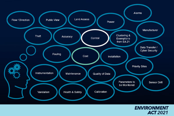
So, when putting together a water quality monitoring program, it is typical to focus on:

• Priority sites, as discussed on the previous slide, locations such as river bathing sites which have a lot of public focus, for example.
• Clustering and exceptions. The current guidance states where discharge outlets are within 250 meters of one another, they can be clustered and monitored by one pair of monitors upstream and downstream. Currently, the one and only exception is if a watercourse has a year-round permanent depth of below 4 centimeters at the optimum monitoring point.
• What parameters you need to measure, and how often. We spoke about the required parameters on the previous slide, and the current guidance states monitoring must be at least every 15 minutes at high-risk times and can be every hour at other times.
• What accuracy do we need? It's still to be defined by DEFRA's technical guidance to monitoring this Act.
• Which manufacturers do we want to work with?
• What instrumentation do they offer?
• And ultimately, what is the cost?

These are the typical thoughts that we initially go through, but we can often miss the much larger and most costly challenges.

• Land access. So, we at Xylem think this will be the number one biggest challenge of implementing the instrumentation for this Act. It's expected a large percentage of sites will not be on water company-owned land, so land access will be a significant challenge. I believe I heard a figure of something like 90 to 95% of all monitoring sites will be on private land.
• Health and safety. So, obviously, water companies do not want their stuff going into rivers on a regular basis.
• The installation of a large number of sites. Obviously, the sheer number of technicians that will be required and their skill sets to deliver a program.
• Theft and vandalism. Obviously, issues created by putting monitoring equipment into the public domain.
• Power requirements, as is expected that most sites will be very remote and will not have access to mains power.
• Fouling, this is one of the most underestimated areas for monitoring, with fouling of sensors increasing the number of visits and maintenance costs.
• Do we need real-time alarms? A smart traffic light alarm system could help water companies quickly identify and action a potential pollution input into a river catchment.
• In an estuary, how do we show upstream-downstream monitoring in a location which has a reverse flow?
• What quality of data are we looking for?
• How often will I need to calibrate?
• What is the acceptable sensor drift?
• What maintenance is needed on site?
• What cybersecurity is in place for these remote devices to be connected to the critical water company infrastructure?
• Do I need to make the data viewable to the public? The current guidance states water quality data must be made public in near real-time, within one hour, and in a common visualization format across England.
• And once I have all this data, how do I use it for spill or pollution prevention control? So, ultimately, how do I turn this data into actions?

 

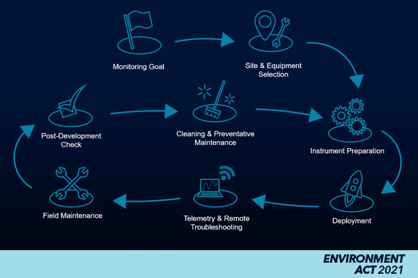
The overall monitoring goal, together with the site and equipment selection, is the single initial cost at the start of any program. Once all of this is put together and the monitoring equipment is all in place, we need to understand the reoccurring costs - the true cost of data. Continual work and costs are required for:

• Instrumentation preparation, so the cleaning of instruments and calibrating them ready for deployment. So, that's lab costs.
• The physical deployment of the sensors on site, so swap in, swap out deployment costs.
• Remote telemetry and a team of people to view, understand the data, to recognize problems or issues. Data analyst costs.
• Going to the field to maintain sites and swap out units, labor maintenance costs.
• Checking the drift of the sensors between visits to understand data uncertainty. Lab costs.
• Cleaning the sensors. And then repeating the whole process again.

To manage a large-scale monitoring program with both believable and actionable data, we need to understand some basic requirements.

Could you take 100 plus of your instruments and be sure that they read the same as each other if all placed in a single tank, never mind the accuracy in the field? Would calibrating the units in the field increase or decrease water quality accuracy? And what levels of uncertainty do you have in your data?

Xylem are the instrument framework provider for the Environment Agency in England, and have worked with them for a number of years to improve the accuracy of data in the field. From this work and thousands of deployments, we've concluded that the best practice should include central laboratory calibration and swap out units.

Sensors should be calibrated with traceable standards, and post calibrations performed to understand drift and uncertainties. This practice has eliminated field-based issues such as cross-contamination, sensor stability, and field labor skillsets, whilst improving the overall data confidence.

 

Now, this is one of my favorite slides I'll show you guys today. The Environment Act Section 82 will produce the world's biggest catchment-wide river water quality monitoring program that there's ever been, generating a vast number of data sets, which we'll need to review, learn, understand, and ultimately turn into information.

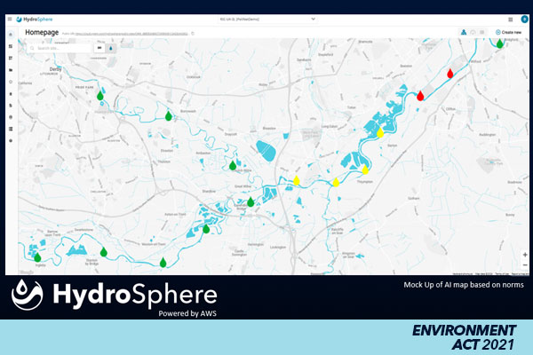
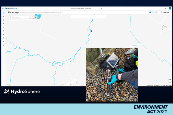
I believe the Environmental Agency mentioned it takes them approximately two hours to review and understand data sets from approximately 200 sites, but they know what they're looking for. This mockup map taken from our cloud-based telemetry platform, HydroSphere, shows how intelligent smart alarms and color visualization can be used to see if sensors are within the expected water quality values, and to quickly highlight the areas for attention. This allows users to be more time efficient with their monitoring program and prevents the user from having to look at data sets from all sites and all parameters on a daily basis.

You can clearly identify straight away from the smart alarm map which site is causing the problem in this catchment, shown by the red dots, and how far downstream it's having an effect, shown by the yellow dots. The ability to recognize catchment and specific site patterns and produce long-term trends for a smart traffic light alarm system and AI will be a very useful tool for water utilities as we move forward with this Act, maximizing the value from their data. The monitoring program isn't just going to show us the potential impacts of storm overflow and sewage effluent, but it's going to provide a national baseline of water quality information for all catchments in England never seen before.

Ultimately, though, it's how we turn all this information into action.

Case Study 01 – Lab Traceability

 

Darren: Thanks, Nate. And as highlighted in the previous slide, monitoring and decision making are only as good as the quality of data which is collected. And with drivers such as the Environment Act, it's common to see some interesting innovations, some new developments, and even some exciting claims. And I really thought that this comment from Yuval Harari really captures the current situation. And I wanted to really take a deeper dive into water quality parameters and their traceability to both known and proven standards.

Water quality parameters really fit into one of three types. And the first type we look at is laboratory replacement. And these are real-time direct measurements in the field which directly compare to those in the laboratory. For the Environment Act Section 82, parameters such as temperature, conductivity, pH, dissolved oxygen, and turbidity, these are all readings which directly compare to results in the laboratory. For ammonia, only a wet chemistry analyzer can directly compare to the best laboratory method.

 

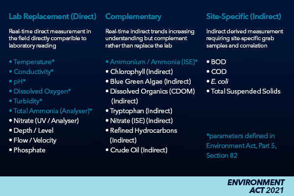
So, although a river-specific ion selective electrode is a direct measurement, there are interfering ions in the water, which means that they fall into the second category, which we consider to be complementary. Now, complementary parameters allow the user to measure real-time trends with their values complementing rather than actually replacing the laboratory measurement. These include ion-selective and fluorescent-based technologies. These parameters can be very valuable for field monitoring, but ultimately, their accuracy is not as good as lab replacement parameters.

The final type of measurement is the site-specific measurements. These are indirect measurements which are derived from the actual values from the complementary sensors, and these require a skilled user to take grab samples in the field, return them to the laboratory, and then create site-specific correlations for that sonde or measurement site. Now, derived measurements have the greatest data uncertainty due to the measurement being based off an indirect complementary method, different user skillsets, and dynamic site-specific interferences.

 

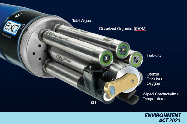
With the YSI EXO, we use smart sensors. And these are truly field-replaceable plug-and-play sensors. These even include wet-mateable connectors. So, if we're out on a typical English rainy day, we can change these sensors in the field in the wet. These can be used in any combination on a sonde to provide customization and comprehensive water quality monitoring. And one of the challenges of the Environment Act is how do we calibrate a lot of sensors en mass? To improve sonde-to-sonde accuracy, YSI developed the multi-sensor calibration method.

Now, with multi-sensor calibration, we can take smart sensors, and they can populate any single sonde to actually calibrate single parameters. So, an example of that would be if you wanted to calibrate six pH sensors at the same time. Now, by using multi-sensor calibration, the user can ensure that all the sensors are calibrated at the same time while saving significant time and calibration buffer costs. As all the sensors hold their metadata for maximum traceability, they know when they were calibrated, who calibrated them, and their sensor diagnosis. This is a real unique innovation from YSI.

 

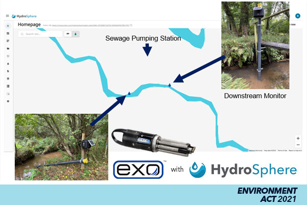
We're going to jump into our first case study. This is a study where we have two YSI EXO sondes. They're installed upstream and downstream of a sewage pumping station. All these sondes were connected to PeliNet telemetry systems, and the data's being pushed to the HydroSphere cloud solution. And as we sort of shown in the previous slides, all the sensors were laboratory calibrated to traceable solutions, and the site visits were every two months for calibration of the ammonia sensor. All data is direct from the sondes, so there's no local calibration here. These are calibrated in the laboratory and then just deployed in the field.

 

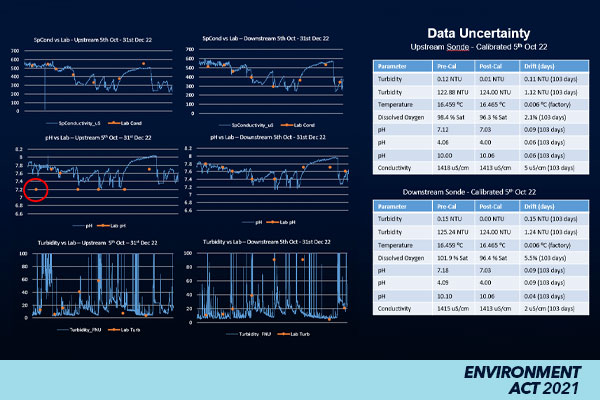
We'll look at the first graph here at the conductivity data. And this is looking at the upstream and downstream data compared to the laboratory. In this situation, the water samples were collected by the water utility and then sent to their accredited lab and then were plotted against the measured parameters in the field.

The next shows the pH. You know, for those with a keen eye on the pH, you'll see that there's one little outlier here, which is showing a lower reading of pH. And what's really interesting when we look at the data, if we see the data versus the laboratory and we compare the upstream and the downstream sondes, we'd actually have quite high confidence here that this is actually an error in the laboratory rather than the field as it's highly unlikely that we'll have a single measurement - that sort of 0.6 pH unit difference - from this downstream sonde in this particular example.

Then, we're going to look at a bit more complicated data. And in this turbidity data, you can see some noise from the sensors. This was actually due to high siltation site creating some fouling issues in the sonde pipe, and that actually required some repositioning to reduce fouling. But I really thought it'd be good to actually show some raw data like this to demonstrate that field measurements do actually come with some challenges.

 After 103 days, the sondes were swapped out and then tested in the laboratory for drift. And when we look at the data, and we see the pre- and the post-calibration data, we can have high confidence that the data that we've collected would actually be good, valid data. We can see good checks against the drift, we can see good checks against the laboratory. So we'd have really high confidence that the data we've collected for these direct measurement parameters would be accurate.

 

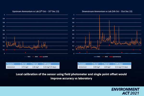
We've taken a look at the lab replacement sensors. So, what about the complementary sensors? Both the YSI EXO sondes were fitted with river-specific ion-selective electrodes. These sensors directly measure ammonium and calculate unionized ammonia using the temperature and the pH sensors. And unlike process ISEs, which we also manufacture, these sensors were designed to be most effective in the lowest range of monitoring. So, in UK rivers, ammonia levels are typically less than 1 milligrams per liter.

These sensors were installed for 73 days with observed drift against the laboratory. So, when we're looking at the upstream sonde, we saw around about 0.25 milligrams per liter and 0.31 milligrams per liter for the downstream sonde. So, that gave us a good indication that the sensors were relatively stable and weren't seeing excessive drift. What we are really also keen to see here is the sensitivity and speed of response because these are critical for effective monitoring. In the laboratory readings (shown here in red) you can see that the ammonia sensor typically reads higher than the laboratory, but these sondes were calibrated using laboratory buffer solutions, so there was no local calibration sonde, this actually came out of the laboratory. And we would recommend here if you wanted to improve accuracy, that a single offset could improve that accuracy.

As we mentioned in the previous slide, the sonde values for ammonium were higher than in the laboratory, and this is because all ion-selective electrodes are subject to interference from ions, which are similar in nature to the analyte. So, these are typically sodium and potassium ions. Due to this interference, these river-specific iron-selective electrodes cannot be used in marine or brackish environments.

Now, the Environment Agency in England has made thousands of deployments using these YSI EXO sondes fitting with ammonium sensors. Based on their testing, they find that a real-world accuracy of +/-0.5 milligrams per liter is what would be expected in the real world. In this particular example, we're using a field offset or against laboratory calibration, and you can see that if we applied an offset of 0.1 milligrams per liter on the upstream and a 0.2 milligram lower offset on the downstream, we'd see that we'd improve the accuracy against the laboratory. So, this is really good indication of collecting good quality ammonium data in the field.

 

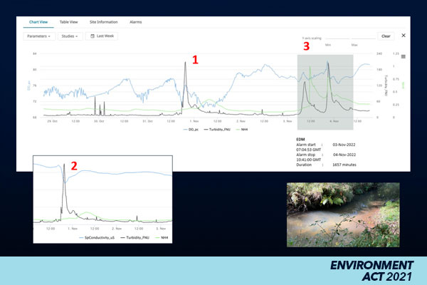
We've looked at the accuracy versus the labs. So, now we're going to focus on the sensitivity of the electrodes. In this dataset - and that's actually from the same site - we observed two large turbidity events, seen here in black. Here, the readings actually exceeded over 200 NTU. For the first observed event, you can see a rapid increase in turbidity but no real change in ammonium. When we look into it a bit further (and add the conductivity data in blue), we can see a drop in conductance at the same time the turbidity increased. This was actually due to a rainfall event which increased the river flow on site. It's likely this turbidity event was caused by runoff and seeing re-suspension of sediments in the water.

The second event shows two distinctive increases in turbidity and a corresponding increase in ammonium, seen in green. The gray box shows when the event duration monitor or EDM was reporting a spill and the corresponding water quality data. It's important to know that although the ammonium in this situation was low, it peaked at 1 milligram per liter, the dataset really shows a clear demonstration of the sensitivity of the EXO river-specific monitoring system, and highlights why the Environment Agency have used these sensors in hundreds of sites in the UK.

Case Study 02 -  Fouling

 

James: For this second case study, we're going to focus on one of the biggest challenges, as we mentioned earlier, for collecting good field data, and that's fouling. Biofouling is a major challenge in any water quality monitoring program. Fouling can create poor data, increase uncertainty, and result in additional field visits and unplanned costs. There are a variety of techniques available to combat biofouling in the field. However, they can be limited by the power availability at the site.

So, low-power anti-fouling techniques for battery or solar-powered sensors and sonde include the use of a high-torque wiper, the use of materials such as sapphire glass, which prevents initial micro fouling, ensuring that all sensors can be cleaned by the wiper, geotextile such as non-woven synthetic weed blocker, copper alloys for use in salt water. If mains power is available, additional techniques can be used, such as a pump flow cell removing the sonde from the light source, UV, air blast cleaning, and ultrasonic. But as you can imagine, these techniques will be limited in remote locations in the field where there's no access to mains power.

For this case study, we'll demonstrate the reasons why we use such techniques.

 

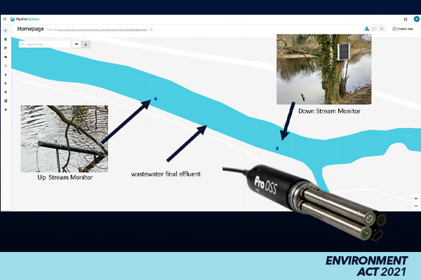
With the number of monitoring sites increasing with the Environment Act, there has been an interest in the use of lower-cost sensors as an alternative to sonde technology. In this example, two YSI ProDSS sondes were deployed connecting to two PeliNet telemetry units. These sondes were installed upstream and downstream of a sewage treatment works. The YSI ProDSS features the same sensor technology as fitted to the EXO sondes but is designed for use as a spot measurement or short-term monitoring device where fouling obviously isn't a concern. 

---

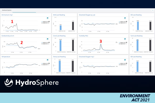
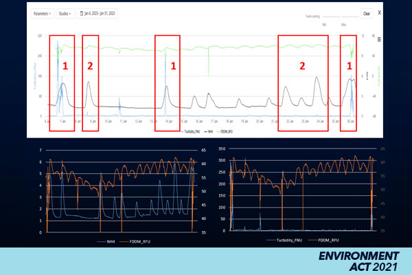
So, here you can see the typical Environment Act user dashboard we've set up in HydroSphere for the water utilities, which compares the upstream and downstream sites in near real-time. The blue line here, or the bar, is the upstream monitor, and the black line, or bar, is the downstream monitor. The data was taken from a trial site in February this year. All data shown throughout this presentation has been collected within the last 12 months. The data from the ProDSS sensors was pretty impressive.

Number one shown here is like a typical sewage-related event as we can see an increase in ammonia content by approximately 1.5 milligrams per liter on the downstream sonde, and that's due to the close proximity with the final effluent discharge. At the same time, you can also see an increase in turbidity and conductivity with a simultaneous drop in dissolved oxygen.

Number two shows a typical rainfall-related event, as we see a reduction in conductivity and ammonium due to the increased flows and dilution in the river. This extra flow reduced the impact on the final effluent on the receiving river, with all readings following the event matching upstream and downstream.

Number three shows a large-scale rainfall storm event. As we can see, there is a significant peak in turbidity detected on both the upstream and downstream sondes, suggesting a turbidity runoff event further up the catchment, so not sewage-related at all there.

 

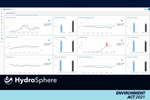
Based on these readings from the 14th of February to the 22nd of February, we can have a high confidence that the data collected was good. This was a great story until a few days later when the downstream sonde detected a large increase in turbidity impacting all the sensors. Following this event shown by number one here, it was observed that the turbidity readings continued to rise on a daily basis. This unusual behavior started to create concerns that the data may not be representative of the river.

The level of turbidity in typical UK rivers ranges from 0 to 50 FNU, and this was peaking at over 1,000 FNU here. So, due to this uncertainty, an additional unplanned site visit was necessary to understand the cause of these readings.

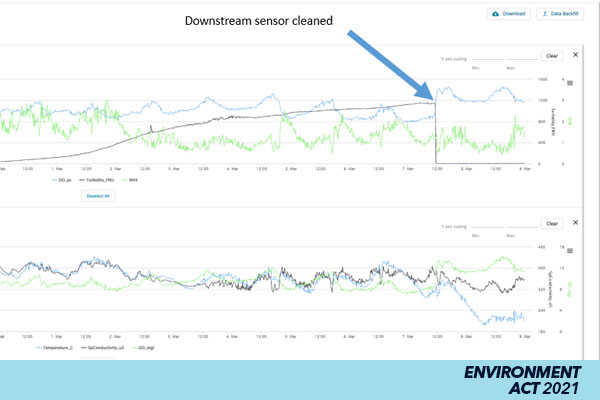
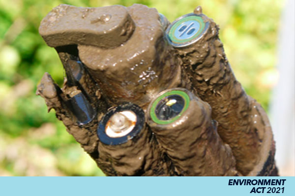
 During this visit, the sensors were removed from the river and cleaned, and you can see by the sudden drop in turbidity, shown by the blue arrow, that the high readings were a result of fouling after just two weeks following the installation. This fouling of sensors creates data uncertainty and raises further questions on the accuracy of the previous data collected from when this heavy fouling event first occurred. It also highlights the time and costs to visit the site potentially every two weeks to ensure data certainty.

 

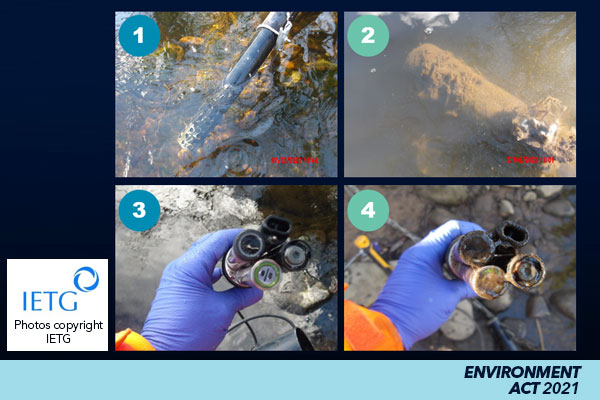
These photos here were taken from the same site, and you can clearly see the problem here. So, whilst the upstream sonde remained clean, the downstream sonde was covered from the incident which impacted the sensors. The use of sensors which are not designed for long-term monitoring in rivers could have a lower initial cost, but increased field visits and higher data uncertainty would make any control or modeling strategy quite challenging.

In this application, we would recommend the use of a YSI EXO sonde with a central wiper to remove the fouling from the sensors. Over time, this will significantly reduce the overall monitoring cost and improve data confidence and accuracy.

For our third and final case study, I'll hand it back to Darren.

Case Study 03 – Derived Parameters

 

Darren: Thanks again. For this final part of our presentation, we're going to look at the complementary and derived parameters. And in this case, we're going to take a look at fluorescent sensors as manufactured by both Xylem and other companies.

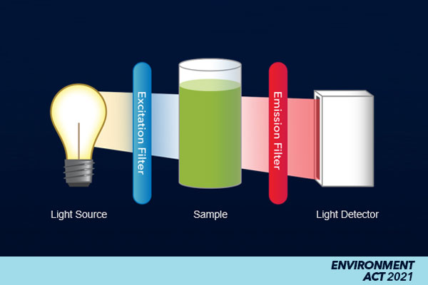
So, all in-vivo sensors operate under whole-cell heterogeneous conditions where the sensors will measure, at least to some degree, everything which fluoresces in the region of a spectrum when irradiated with a specific wavelength of light. Common uses of these sensors includes chlorophyll, rhodamine, blue-green algae, crude oil, refined fuels, tryptophan, and colored dissolved organic matter. Each one of these sensors has a minimum detection limit, and this can sort of vary between different manufacturers. But it is important to note that these sensors are best employed as qualitative, complementing laboratory, but not replacing laboratory. And one of the reasons why these are best used for trending is due to potential interferences, including temperature, turbidity, and as dissolved organics.

Unfortunately, these parameters are the same parameters which typically increase during storm overflow events. It is actually impossible to exclude interference from other fluorescence species by just using a simple lab calibration. So, we can't just calibrate it in the lab, put it in the field, and then get a good measurement. That means that we have to go to the site, we need to take grab samples, and for those using those grab samples, we'll form a local calibration or a best-fit algorithm to suit that site.

But even then, it's unlikely that the grab samples that are taken at a specific site will be there when these different interferences are present. Therefore, local calibration still has some considerable uncertainty if we're trying to take these values and convert them into derived parameters such as BODs, suspended solids, total algae, or E. coli using best-fit algorithms or single local samples. But it is important to note that when used correctly and the uncertainties are actually understood, the use of fluorescent sensors can be a valuable addition to any monitoring program.

 

So, we're going to take a look at a case study here. This is actually looking at combination or direct measurement of laboratory parameters and fluorescent sensors. In this case study, we're looking at final effluent from our wastewater treatment works, and we're measuring temperature, conductivity, pH, turbidity, dissolved oxygen, ammonia ammonium, and dissolved organics. Like in previous studies, all of the sensors are fitted to EXO sondes, connected to PeliNet telemetry systems, and collecting and transmitting data every 15 minutes.

Now, when we look at the data we see here, this first event was really interesting, and the data shows an increase in ammonium from 4.5 to over 7 milligrams per liter. We can see in this study that the actual organic sensor responded well with this event. And in isolation, we could look at this and say, this is clear evidence for the use of CDOM as a surrogate for ammonium. And, when we first looked at them, and think this really exciting data, so we kept running this study, and as a study progressed, we see a second set of ammonium peaks, this time raising from 2 to 4.5 milligrams per liter.

 

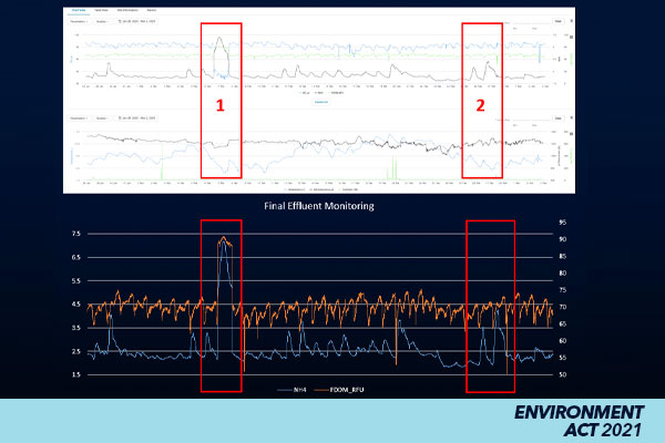
However, in this situation, we see no response from the dissolved organic sensor. Now, here we could take grab samples, we could form a correlation around the baseline of this data, but it's about this sort of sensitivity around alarming and actually seeing events which we're most interested in. And when we don't know if we have good sensitivity or good selectivity, that creates further uncertainty. So, again, as we looked into these sort of numbers, ammonium in a typical river is less than 1 milligram per liter. But in this data set, an increase of 2.5 milligrams per liter, which the Environment Agency would actually consider to be an event, was actually undetected by the fDOM sensor.

So, we followed on from this, and we started looking at the previous month's data. In the top graph, you can see the ammonium data in black from the YSI EXO sondes. We can see here good response and nice clean data from the sensor. And then, we focus on the turbidity data, which we can see here in blue. At this site, we can see that some of the increases in ammonium are actually when turbidity increases to over 100 NTU from the works. These large increase in turbidity have caused a dissolved organic sensor to decrease its readings due to these interferences.

We can see these little drop-offs each time we see the turbidity increase. So, if we installed just the dissolved organic sensor on the final effluent, we would have, on some occasions, shown lower readings at a time when increased ammonium was actually happening on the discharge. We'd be seeing the opposite from our sensors of what's actually seen in the field. Now, in these events, the ammonium readings have actually increased from 2 to 6 milligrams per liter. This is a significant increase in ammonium, but again, it wasn't detected by the fDOM sensor.

 

So, although data can be improved by grab samples and local correlation, this data is just further evidence that fluorescent sensors should be used for trending only. Matrix calibrations, they're not dynamic, so, they can't adjust for interferences in real time. So, when we use dissolved organics, we look at using them as an additional parameter. And we have to say that, because of the way that we're measuring, we could have further uncertainty in our measurements. So, it's really important when we're trying to look into those parameters which are traceable, and those parameters are giving us a very interesting information, we'll have some certain level of data uncertainty.

Let's look at the positive. And so, although it's an indirect measurement, fluorescent sensors are simple to add to any EXO sonde using a field-swappable plug-and-play digital sensor. And as shown in the previous study, no fluorescent sensors on the markets today actually feature dynamic correction. So, unless we're deploying in a low turbidity application such as groundwater, all measurements will have inaccuracy regardless if site-specific calibrations were made. But, if limitations are actually understood, and the user wishes to see just relative change, these sensors do provide valuable complementary information, which can benefit any monitoring program.

It's shown here that YSI really recommends reporting these values as relative fluorescent units or RFU. This helps eliminate any misinterpretation of a derived parameter to being read as a measured parameter on a report. So, we're obviously looking at data in real time, but we are also aware that this data will be viewed over time as well. So, we think it's important to actually output what we're measuring as opposed to what we're deriving.

 

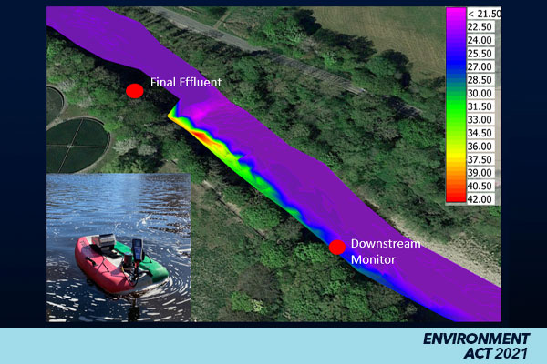
As well as sort of continuous measurements, these sensors can actually be used for both mixing and for tracing studies. In this example here, we're showing a Xylem rQPOD. It's a remote-controlled vehicle, and it's fitted with EXO sonde. And this is spatially measuring water quality from a final effluent discharge. This map is showing data from the fDOM sensor, and this data is extremely useful to understand the mixing of the final effluent of the river water or tracing sources of pollution. As you can see in this particular example, the downstream monitor is still actually monitoring a little bit of the final effluent from this site.

And when we're looking at the Environment Act Section 82, we're trying to measure the impact on the river, not the actual effluent itself. So, in this particular situation, we're showing that the downstream monitor is actually cited a little bit too close to the final effluent, and we'd recommend actually moving that. So, note that these parameters are all in relative fluorescent units. So, if we wanted to show these values as any of the derived parameters, we would need to take grab samples, and we would have to do a site-specific calibration.

But like with the spatial measurements, these are really spot measurements, and local calibrations will only represent a single point in time. So, if we add dynamic events such as floods, runoff, or spills, that could actually impact the matrix model and no longer be representative. And it's really due to these factors that we would state that all fluorescent sensors complement rather than replace the laboratory.

Conclusions

 

James: Thank you for that interesting presentation, Darren. And we're just going to follow on for today's presentation. We're just going to conclude some of the things that we've just spoke about.

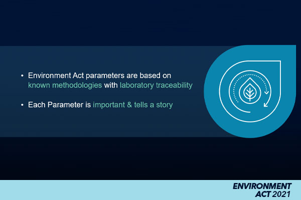
So, the Environment Act parameters are based on known methodologies with laboratory traceability. River water quality is dynamic and is constantly changing. So, each of these Environment Act parameters are important and have a role to play as they interact with each other and can tell a different story each time.

New innovations in sense technology will benefit the environmental monitoring sector, but more testing is needed. A good understanding of lab traceability, fouling, and known interferences will be required to assess current market offerings and new innovations. Centralizing calibration to known standards will help to normalize data across catchments, as demonstrated by the Environment Agency’s National Water Quality Instrumentation Service. And for best practice, field calibration should be avoided if possible due to potential errors, skills gaps, and health and safety concerns.

 

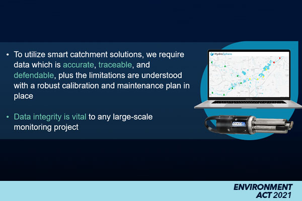
To utilize smart catchment solutions, we require data which is accurate, traceable, and defendable. Plus, the limitations need to be clearly understood. This needs to be backed up by a robust calibration and maintenance plan in place. Intelligent traffic light alarm systems and artificial intelligence could be the future to maximize the value from this data. Data integrity is vital to any large-scale monitoring project. If you can't monitor accurately, you cannot manage or action the data that these systems can provide.

YSI has been established since 1948, with the first multiparameter sonde being released in 1992. The EXO-S Range is the fifth generation of sonde from YSI, and have been solving water quality issues in the field for many years. We have used this experience to understand what goes wrong in the field, and design sondes to ensure reliable, accurate, and traceable data.

Thank you for listening and attending the webinar today.

Nate: Thank you, everyone. So, we're going to start the question-and-answer portion of the webinar in just a minute, but first, I wanted to point out a few additional resources. If you're interested in learning more, you can check out ysi.com/environment-act-2021. This will be our home for all things related to the Act. You can learn more about the recent legislation, water quality sensors, and view additional webinars and other resources to help get you started with monitoring in the field.

 

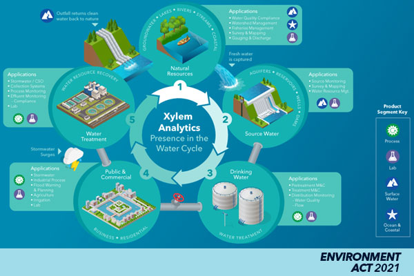
We also wanted to remind you that no matter where you are in the water cycle, Xylem is here to help. We have solutions for surface water, natural resources, source water, drinking water, public, commercial, and water treatment.

Alright, so now let’s take a look at the questions that have come in so far. Catie, do you have any questions you’d like to get us started with?

Q&A

Editor’s Note: The Question and Answer portion has also been abridged. For the full Q&A, please watch the recording starting at 43:26.

Catie: Yeah, I'm going to go ahead and kick it off with a comment Kent put into the chat about doing DO calibrations in the field because barometric pressure can differ between field and lab. And yes, you're absolutely correct there, some calibrations might be better to do in the field. The EXO sonde is designed to be used or calibrated in the field as well as the lab. So, it's really up to your SOPs, you know, your standard operating procedures. That's what we recommend you follow.

Our recommendation for this presentation for calibrating them in the lab was based on these practices specific to the studies performed here. So, calibrating in the lab can absolutely help you reduce contamination. Just like Darren was saying and James, it can be an alternative to calibrating the field. If you find you have specific issues related to field calibrations, you can make sure that you're limiting contamination in your standards when you're doing your calibrations. Make sure that all the people in your group are performing calibrations the same way, and help you standardize your procedures. But absolutely, the EXO can be calibrated in the field. There's nothing wrong with that. And Darren, do you wanna add anything to that?

Darren: Yeah, of course. One of the reasons why something like DO is measured in the laboratory in the UK is more to do with getting data that they know is repeatable. So, one of the things we look at for barometric pressure and the actual inaccuracy for barometric pressure, that's seen as a smaller error versus the potential of calibrating in the field. You know, it's one of the reasons why they calibrate that way is because we are calibrating centrally. And if I take the Environment Agency practice, you know, they'll be shipping out hundreds of units around the country to monitor.

And they really need the user at that and to be able to collect the sonde, go to the site, just swap the sonde over in the site. And so, as soon as we start getting into field calibrations, we need different training, we need different methodologies. So, it's been found over the years that actually calibrating in the laboratory in that situation and understanding the potential uncertainties caused by barometric pressure would be acceptable.

Catie: Absolutely. So, it's really based on your needs, your calibration needs, your procedures. So, just following whatever works best for you guys is definitely what will be most beneficial.

---

That's really going to depend on the sites. Having a central wiper installed on your EXO2 or EXO3 will definitely help reduce fouling issues, keep those sensor faces wiped clean. We have other anti-fouling methodologies that will help reduce fouling over time, like a copper sensor guard, copper tape for your sensors, using just duct tape even to duct tape your sonde up. We also have heat shrink wraps for the sensors and the sonde. So, they're plastic sleeves that you can apply to your sonde before deployment.

And then, during deployment, if you have biofouling buildup, you just cut that tape or the heat shrink sleeves right off, and then you're starting over with a clean sonde again. So, those can be really helpful. There's also C-Spray that can reduce fouling by kind of making the surface of the sensors and the sonde slippery so that biota can adhere to it. But as far as the frequency for cleaning, it's really, again, going to depend on your site, how bad your fouling is, what kind of methods you're already using, what type of fouling you're experiencing, whether it's barnacles, algae, debris, sediment.

---

And speaking of calibrations, I'm just going to go ahead and jump into a question on how often to calibrate. And that's one that we get pretty often.

How often you calibrate is really going to come down to, again, your standard procedures, what works best for you, your team, and your sites. It can depend on the age of your sensors, the modules that you're using, whether your DO cap is new or has been in use for a year, as well as your pH module. Those are interchangeable so the age of those modules matters. And then your calibration practices, whether you're able to limit contamination during your calibrations, how much fouling you're getting, the environmental conditions.

So, just keep an eye on your data. If you're experiencing a lot of drift over time, maybe you want to increase the frequency at which you're calibrating your sensors to reduce that drift. Optical sensors like DO and Turbidity tend to be more stable over time, they experience less drift compared to, say, electrochemical sensors like pH, which tend to be more prone to drift. So, it depends on the sensors you have.

But our benchmark, what I like to recommend to people, is the monthly calibration of your sensors. It's a good place to start. You might need less frequent calibrations than that. And that might be fine for your sensors and, you know, you experience minimal drift just like Darren showed in this presentation. Two months of a period of time between calibrations worked really well, and they had very minimal drift. That's absolutely great. But if you're seeing more drift than that, you have an environment that requires more calibration, then absolutely, calibrate more frequently if that helps keep your sensors stable.

Darren: The important thing itself is the data, you've got to have confidence in the data. As soon as we're in a situation where we don't know if that data's good or bad, we've lost because now suddenly we've got a lot of uncertainty, and that's what creates a lot of issues on projects.

Catie: Right. That's kind of the fun part of environmental field monitoring. You know, you have to do troubleshooting on the job. You have to do the best you can to understand your site and the possible barriers that you may be facing.

And kind of in line with that, we have a question: What is the useful life of the sensors? And this is referring to each of the EXO sonde sensors. We have several different options: pH, turbidity, DO, etc. So, we're referring to what is the life of those sensors, and it really could be as long as, if you keep up good maintenance and calibration of them, they may last 10-plus years, just like a lot of people using the 6-Series Sondes, which is the precursor to the EXO.

Those have been in the field for 30 years and still going strong. It really depends on the environmental conditions. If you have a lot of fouling over time or if you're in heavy fouling conditions, salt water, and having issues without being able to do very frequent maintenance, if you have a lot of buildup, it might damage the sonde over time. So, again, staying on top of maintenance can make your sensors last longer. I've seen five to seven years is a really good benchmark for that, but again, could be much longer than that.

And conversely, it could be shorter if you're not keeping on top of lubricating your sensors. All the sensors for the EXO have wet-mate connectors. So, what that means is they can be swapped in and out with moisture present in the pods, and that's totally fine. There'll be no issue with operation of the sensors if there's moisture in the pods. And that's because the pins are protected with neoprene rubber on each of the pods. But that neoprene rubber needs to be kept moisturized.

Every EXO and sonde sensor shipment comes with Krytox lubricant grease, and we use that to keep those rubber connectors lubricated. And you should be doing that every time you calibrate your instruments. Take the sensors out, lubricate them, clean any debris out of the O-rings, and from the threading, reapply fresh lubricant and reinstall. And that'll help extend the life of your sensors a lot. So, those are definitely really good things to keep in mind.

I have an interesting question. So, this is regarding HydroSphere. We showed some examples for kind of illustrative purposes. What are you basing the thresholds for the red, yellow, green? And those were for the droplets that we showed on the map.

HydroSphere allows you to personalize the alarms you set. So, you can have alarms set for whatever thresholds you want based on any of the parameters that you have coming into HydroSphere. And again, HydroSphere is the data platform that is accepting parameter data from the sondes. So, any of that uploaded data can be set to display alarms and they're totally customizable. So, I don't know what the red, yellow, green was for your specific map, Darren, if you remember what those are based on.

Darren: What we've been doing with the trial work with the water utilities in the UK is sort of agreeing what those limits would be. And the way that we do this is we supply a Smartsheet to those customers who will actually say, "Well, if we don't agree with those parameters or we wanted to look a little bit tighter," they can provide them to us. And then, by the sensors looking at all of the different parameters and all the different outputs, including any sort of hardware issues, the sensors will just be able to just give you that color output.

So, as Catie says, it's customizable. I think really for the Environment Act, it's going to be water framework directive based around the actual tolerance limits. But we have had some sites, which we have naturally quite high conductivity and where those standard parameters that we've been using would give it in a red alarm. So, we've had to tweak those red alarms on those particular sites because they've got a natural river conductivity of around about 1,000 microsiemens as a good example.

And it's a similar thing when we look at ammonia. Ammonia is an important one because we'll look at the consent of a treatment works, but consent is for the concentrate coming out of the final effluent. And then when we're looking from an Environment Agency point of view is looking at the impact of that diluted effluent in the river. And so, normally, those values will be considerably lower than the sort of final effluent discharge when we're monitoring further downstream.

And you saw from one of the examples there, if we monitor too close to the final effluent, we all see higher levels of ammonia than actually are being diluted into the river. And that can give us a false positive because, obviously, we know that there are higher levels of ammonia coming out to the final effluent. What we need to understand is how it impacts the watercourse. So, these are just some examples of how we can actually tweak things really as needed.

And in those applications, we wouldn't recommend an ion-selective electrode. So, really, think of it as a fresh water-only probe. Going into saltwater applications, we'd more likely use an analyzer for measuring the ammonium.

Nate: Yeah. Here's a good one for you, Darren or James. They want to know if you've tested the EXO's in a pumped kiosk solution and how does the data compare to a direct river application?

Darren: Yeah, that's a great question. Pump kiosks work extremely well in applications where you've got very shallow water or the distance between the actual bank and the river is greater than about 5 meters. Then, pulling the sample up for a flow cell and putting the EXO directly into a flow cell can work extremely well. The challenge that you face in this is not the methodology because the methodology works fantastically. By keeping the sensor in a dark environment, in a flow cell, we also see minimal biofouling.

The challenge tends to be power. So when we're putting in a pump flow cell system, you can either use solar panels, and they could be fairly large solar panels. In certain areas which may attract either theft or vandalism, they can be problems. Or we can use things like methanol fuel cells. The methanol fuel cell works as a power generator charging up the battery. Again, these work really, really well. But we've now moved a challenge over to carrying and transporting methanol fuel cells in the field. So, generally, whichever methodology we use, there's always a challenge to overcome.

So, if we have sondes, they are designed to go into the river directly, but by being in the river directly, there'll be certain elements of fouling or parts that could cause issues. If we're in very shallow water, let's say the water's only a few centimeters deep, it can be difficult to get a sonde directly into that application, and a pumped flow cell and a strainer with a sort of reversible pump can work really well. So, a good example would be the Environment Agency. They've got a number of flow cell applications out there collecting extremely good data. I mean, flow cells work really, really well with EXO sondes.

Catie: There's one more question I want to get into, and this question was regarding facing an issue with their EXO sensor, having a broken pin after a year of use. And I do want to mention that the sensors for the EXO - they're titanium build - they're meant to last a long time. They have a two-year warranty. So, if you have issues with your sensors, please reach out to us. You can reach out to info@ysi.com. That's just a good place to start. That's the tech support line, but you can be directed to repairs or your local sales rep as needed to help you out with any issues. But as far as any performance issues with your sensors, things that aren't performing as they should be, please reach out to us and we'll get those concerns taken care of.

---

Catie: Yes, we can absolutely follow up with you individually, for anything we missed.

Nate: That's a great point. If we didn't get to your question, we will make sure to follow up with you soon.

We want to thank you all so much for joining us for the webinar today, especially with it running a little long. We really appreciate all the interaction, all the engagement. We hope it helps you feel more prepared to gather high-quality, reliable data in the field. So, wherever you are in the world, from everyone here at Xylem, we wish you lots of success in your environmental monitoring efforts. Thank you.

---